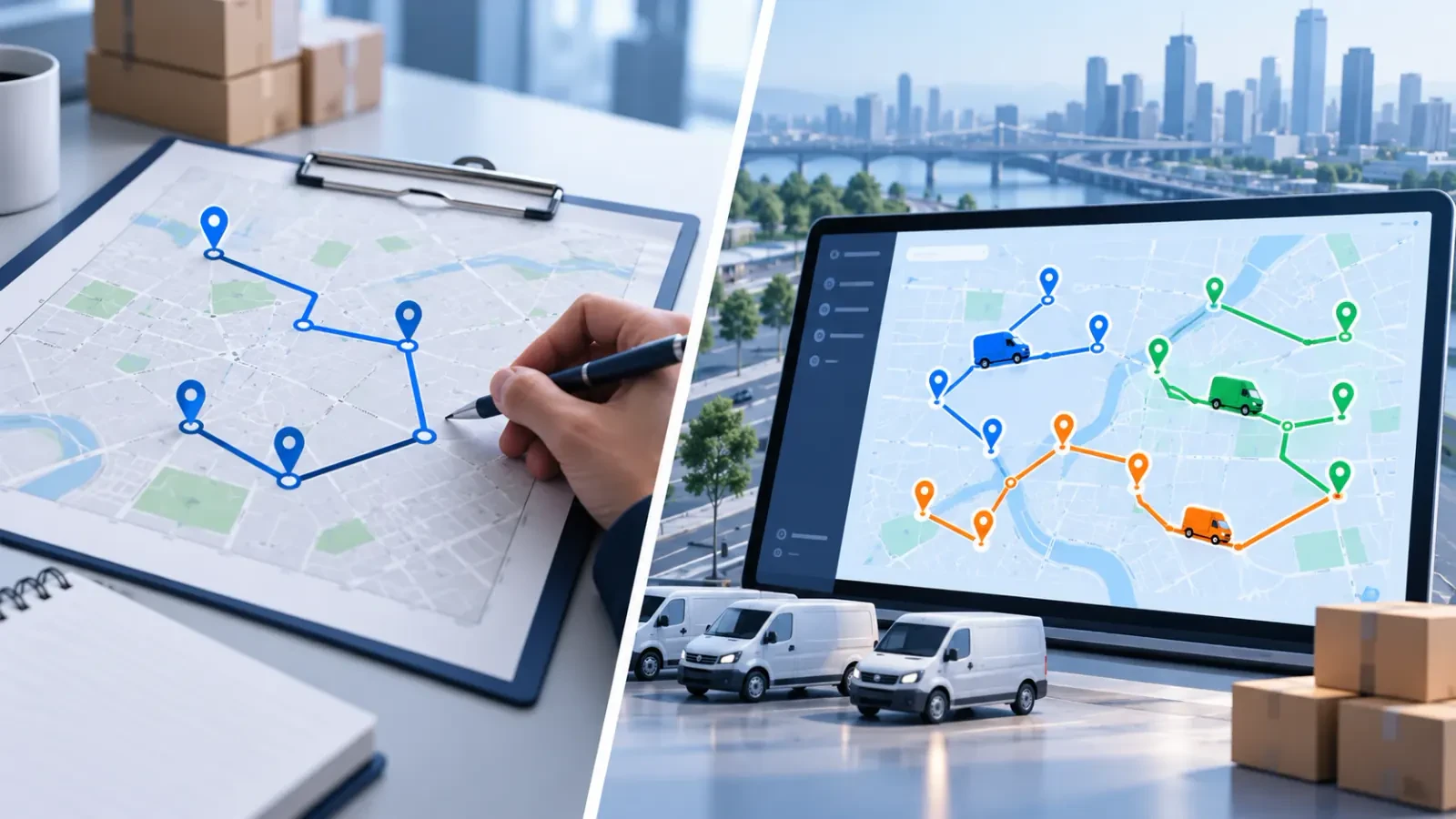

In a delivery operation, finding the shortest route is not always enough to build a successful delivery plan.
A vehicle may be sent to the right customers, but if it exceeds its load capacity, the plan cannot be carried out. Likewise, a route that looks good in terms of distance may fail the operational requirements because it misses a customer’s delivery acceptance hours.
That is why route optimization considers two important elements together: vehicle capacity and delivery time windows.
In this article, we look at how these constraints affect route planning, how mathematical optimization models handle them and what businesses should watch for while planning, with examples.
How does vehicle capacity affect route optimization?
Vehicle capacity is the amount of load a vehicle can carry. In route optimization, this limit is one of the basic constraints that decide which vehicles tasks can be assigned to.
The Capacitated Vehicle Routing Problem (CVRP) covers route optimization problems in which vehicles have limited load capacity.
In the classic CVRP, the goal is to build routes that satisfy customer demands without exceeding any vehicle’s capacity. The objective is usually defined as total travel distance or a corresponding cost. [1]
Capacity is not only about weight
In logistics operations, capacity can be expressed in different measures:
- Weight: The limit on the load a vehicle can carry, in kilograms or tons.
- Volume: The total volume of the goods that can be carried.
- Pallet capacity: The number of pallets that fit in the vehicle.
- Item count: Boxes, crates or similar units, depending on the operation.
Staying below a vehicle’s weight limit does not by itself guarantee that the load will physically fit.
For example, a vehicle with a 1,000 kg limit and 10 m³ of usable volume may not be able to take goods that weigh 800 kg but occupy 12 m³.
So a suitable optimization model can evaluate several capacity dimensions together. PyVRP offers examples of modeling capacity constraints with more than one load dimension. [2]
There is an important distinction, though: meeting weight and volume limits does not always prove that the goods can be physically arranged correctly inside the vehicle. Three-dimensional loading, product compatibility and stacking rules are separate problems that need their own modeling.
What is a delivery time window?
A delivery time window defines the interval in which a customer can receive a given service.
For example, if a store accepts goods only between 09:00 and 11:00, planning has to take this interval into account.
The Vehicle Routing Problem with Time Windows (VRPTW) covers planning customer visits within specified time intervals. [3]
Arriving early and arriving late are not the same
A vehicle can reach a delivery point before the allowed time.
For example, if a customer starts accepting service at 10:00 and the vehicle arrives at 09:40, then under the conditions the model allows, the vehicle can wait 20 minutes and start service at 10:00.
On the other hand, if the vehicle misses the latest time defined for starting service, the route may fail the constraint.
It helps to separate three different time concepts here:
- Arrival time: The time the vehicle physically reaches the delivery point.
- Service start: The time loading, unloading or the delivery itself begins.
- Service end: The time the work is completed.
In some optimization models the time window limits when service starts. In such a model, service can start before the window closes and finish afterward. But if the customer needs a deadline by which the delivery must be fully finished, that has to be modeled separately and correctly. [4]
This distinction matters for carrying real-world delivery commitments over to the mathematical model accurately.
Why should vehicle capacity and time windows be evaluated together?
A plan can be fine in terms of capacity and still fail the time constraints.
Likewise, a task assignment that reaches every customer on time can exceed the vehicles’ load limits.
Evaluating these constraints independently can therefore produce plans that cannot be carried out in the field.
For example, assigning two nearby customers to the same vehicle can look sensible in terms of distance. But if their delivery times overlap and the travel and service times between them cannot be shortened enough, the tasks may have to go to different vehicles.
That is why it matters for the optimization algorithm to evaluate not only the visit order but also which customer is visited by which vehicle, and at what time.
Example: Planning four deliveries with two vehicles
To make this concrete, let’s set up a representative delivery operation.
The business has one depot and two delivery vehicles.
| Vehicle | Load capacity | Departure from depot |
|---|---|---|
| Vehicle 1 | 700 kg | 08:30 |
| Vehicle 2 | 500 kg | 08:30 |
The deliveries to be made to four customers on the same day are:
| Customer | Load | Delivery time window |
|---|---|---|
| A | 400 kg | 10:00–10:30 |
| B | 300 kg | 09:00–09:30 |
| C | 250 kg | 09:00–10:00 |
| D | 200 kg | 10:00–11:00 |
| Total | 1,150 kg |
The total capacity of the two vehicles is 1,200 kg.
Although the total load is below this limit, that fact alone does not prove all tasks can be distributed properly. The individual capacity limits of the vehicles and the delivery times also matter.
Step 1: A task assignment that fits capacity
Consider this assignment:
Vehicle 1: Customers A and B — 400 + 300 = 700 kg
Vehicle 2: Customers C and D — 250 + 200 = 450 kg
Neither vehicle exceeds its own capacity limit.
But this does not mean the plan is finished. Now we need to check whether the delivery times are met.
Step 2: Evaluating the time windows
In our example, let’s assume the following travel times:
| Route | Travel time |
|---|---|
| Depot → B | 20 minutes |
| B → A | 30 minutes |
| Depot → C | 20 minutes |
| C → D | 20 minutes |
Assume the delivery at each customer takes 10 minutes and the vehicles can leave the depot at 08:30.
A possible plan for Vehicle 1
| Time | Action |
|---|---|
| 08:30 | Departs from the depot |
| 08:50 | Arrives at customer B |
| 09:00 | Starts the delivery |
| 09:10 | Leaves customer B |
| 09:40 | Arrives at customer A |
| 10:00 | Starts the delivery |
| 10:10 | Completes the work at customer A |
Vehicle 1 meets the delivery time windows of both customers.
Since it arrives 10 minutes early at customer B and 20 minutes early at customer A, it waits at each.
A possible plan for Vehicle 2
| Time | Action |
|---|---|
| 08:30 | Departs from the depot |
| 08:50 | Arrives at customer C |
| 09:00 | Starts the delivery |
| 09:10 | Leaves customer C |
| 09:30 | Arrives at customer D |
| 10:00 | Starts the delivery |
| 10:10 | Completes the work at customer D |
Vehicle 2 also meets the defined time windows.
So the task distribution of the two vehicles looks suitable in terms of both capacity and customer service start times.
However, we should note three important points about this scenario:
- Only capacity and the given time information were checked here.
- The vehicles’ return times to the depot, other working limits and the real road network were not evaluated.
- The resulting plan was not shown to be the lowest-cost or shortest-distance solution possible.
This example is a representative scenario prepared to explain the concepts. It is not a result calculated by a real optimization algorithm or taken from a customer’s operation.
How do time windows change the route sequence?
In the example above, note that Vehicle 1 visits customer B first and then customer A.
Customer B accepts deliveries between 09:00 and 09:30, while customer A accepts them between 10:00 and 10:30.
If the vehicle went to A first, service at A could start at 10:00 at the earliest. Going to B after that would miss B’s window, which ends at 09:30.
So the visit order of the two customers should not be decided by geographic proximity alone.
The effect of time windows on routes has long been studied in vehicle routing research. Solomon’s 1987 paper is one of the foundational academic studies on heuristic methods for vehicle routing and scheduling problems with time windows. [5]
What happens when capacity and time constraints cannot be met?
A solution that serves all tasks may not exist for every planning problem.
For example:
- The total load may exceed the carrying capacity of the available vehicles.
- An order may not fit into any of the suitable vehicles.
- The time windows of two deliveries may be too narrow to assign to the same vehicle.
- The available hours of vehicles or drivers may not be enough.
- The mandatory assignment rules set for tasks may conflict with one another.
In this case, running the algorithm for longer does not always produce a solution.
First, you should check whether the problem actually has a feasible solution.
Depending on the business’s operating rules, alternative approaches can include:
- Using extra resources: Increasing the available vehicle or driver capacity.
- Rescheduling tasks: Moving deliveries to other times or days if customer conditions allow.
- Splitting tasks: Distributing suitable orders over more than one transport trip, only if the operation allows it.
- Identifying unserved tasks: If the model allows it, leaving some tasks out of the plan and evaluating the cost of doing so.
One method used in the optimization literature for the last approach is to assign a penalty cost to customers that are not visited. Google OR-Tools provides examples of this approach. [6]
However, skipping the delivery of a critical customer may be unacceptable for the business. So it must be defined clearly which tasks are mandatory and which are optional or can be postponed.
Why do errors in planning data matter?
The results an optimization algorithm produces depend on the accuracy of the data and the model.
For example, if a vehicle can really carry 500 kg but is defined in the system with a 750 kg capacity, the algorithm can build a plan that is valid according to its own data but physically impossible to carry out.
Similarly, if a customer’s delivery acceptance hours are entered wrongly, a plan that looks valid in terms of time will not be enough for the real operation.
So before planning, check the following in particular:
- Current load capacities of the vehicles
- Quantity and load information of the orders
- Correct locations of the delivery points
- Customers’ acceptance hours
- Service time per stop
- Vehicle and driver availability
- The travel time estimates used
Improving data quality can, in some cases, bring a more meaningful improvement than making the optimization model more complex.
Which performance indicators matter for businesses?
To assess how vehicle capacity and time windows affect planning, total kilometers alone should not be the measure.
Different indicators can be tracked depending on the business’s goals.
Capacity utilization rate
Shows how much of the vehicles’ usable load capacity is used.
A simple example, calculated from the quantity loaded at the start:
Capacity utilization rate = (Loaded quantity / Vehicle capacity) × 100
For example, if 630 kg is loaded onto a vehicle with a 700 kg capacity:
630 / 700 × 100 = 90%
But this rate alone does not prove the operation is efficient.
In operations where pickups and deliveries are done together in particular, the vehicle’s load can change along the route. Weight and volume utilization rates can also differ.
Time window compliance rate
You can track the share of deliveries carried out within the defined service time windows.
Time window compliance rate = (Number of deliveries within their time window / Number of deliveries evaluated) × 100
It should be defined in advance whether the measurement is based on service start or on completion of the delivery.
Total tasks and route duration per vehicle
How many deliveries vehicles make and how long this takes can be evaluated together.
However, it is not correct to say that a vehicle making more deliveries is always more efficient. The distance between delivery points, handling times and vehicle characteristics must be part of the evaluation too.
Waiting times
Waiting time caused by customers’ acceptance hours is an important time component in route planning.
Analyzing waiting times can help you understand better how time windows affect the route.
How does mathematical optimization handle these decisions?
In vehicle routing problems where capacity and time windows both exist, the optimization model evaluates the assignment of tasks to vehicles and the visit sequence of stops together.
For a solution to be considered valid, all constraints defined as mandatory in the model must be satisfied.
For example:
- Capacity condition: The load a vehicle carries along its route must not exceed its defined capacity.
- Time condition: At each customer, service must start within the time interval defined in the model, or meet the other timing rule set by the business.
- Task condition: Mandatory deliveries must be carried out according to the defined rules.
Once these conditions are met, the algorithm can try to improve the value of total distance, travel time or another objective function.
In large and complex problems, finding the mathematically proven best solution can be difficult. For this reason, heuristic and metaheuristic methods are used to obtain good solutions in practical computing times. [5][7]
How does Trackinia handle these planning needs?
Trackinia is a logistics operations management platform that evaluates route optimization together with vehicle and driver planning.
Operational conditions such as vehicle capacities, delivery time windows, resource availability, working hours and task assignment rules can be taken into account in planning.
In daily and multi-day planning scenarios, the aim is to distribute tasks to suitable resources and days.
Plans can be reviewed on a map and a timeline. This lets operations teams evaluate the optimization result and relate planning decisions to their existing workflows.
To see how capacity and time constraints affect route planning in your business, you can request a Trackinia demo based on your current delivery structure and operational needs.
Conclusion
Vehicle capacity and delivery time windows are among the core elements of route optimization.
Capacity constraints determine which vehicles can carry out which tasks, while time windows limit when those tasks can be done.
When these conditions are evaluated together, the aim is to prepare plans that meet real operational requirements instead of merely producing short routes.
A successful route optimization process needs accurate data, suitable mathematical models, clearly defined business rules and an operational evaluation of the results.
One of the main reasons the shortest path is not always the most suitable plan in route optimization is that businesses work under physical and time constraints.